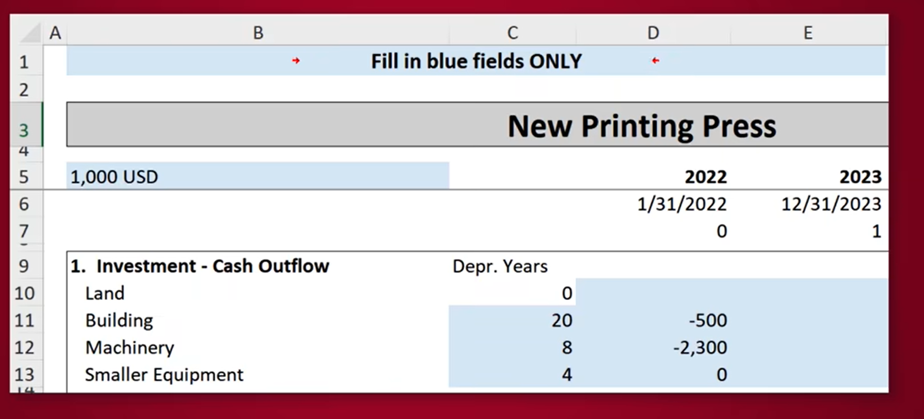
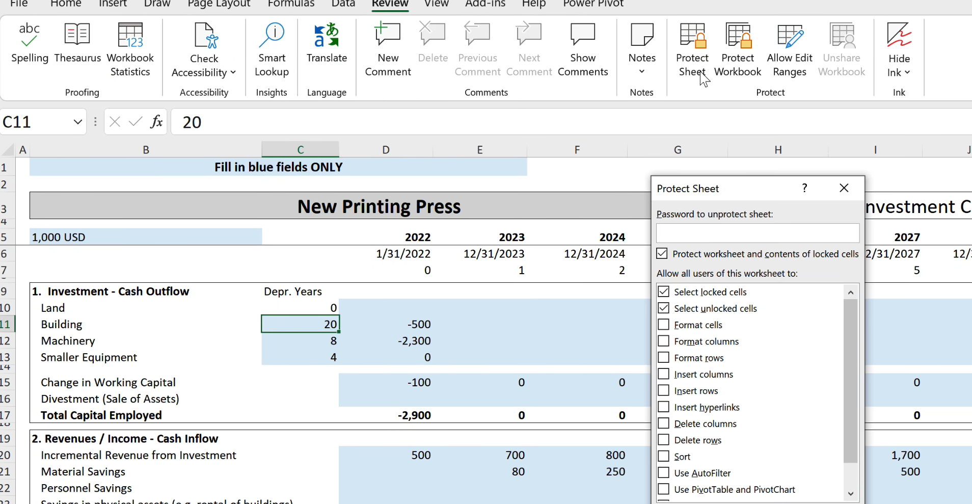
As an Excel user, you may have come across the term column lock while working. But do you really understand what it means? And how to lock a column in excel tough? Here below, we will look at concept of how to lock columns in excel and how you can use it to your advantage.
Table of Contents
how to lock a column in excel
Excel column lock refers to freeze or lock specific columns in place while scrolling through spreadsheet. This is especially useful when you have a large spreadsheet with multiple columns. In this way, you can for example freeze headings. But you can also check your long list as you scroll. If this is a student list for example, you can see the heading student name and number at top.
excel column locking: What Is Excel Column Lock?
For example, you have your customer data. And it is including their names, addresses and purchase history. If you want to keep the customer names visible while scrolling through the rest of the data, you can use excel column locking to freeze the first column in place.
Hence, you can easily reference the customer names as you work with the rest of the data.

how do i lock a column in excel:how to lock columns in excel
Now that you understand the concept of column lock. It is time to take a look at how you can lock columns in Excel. How you do it is actually depending on your preference. As well as Excel version you are using is important here.
Method 1 for excel locked columns: Freeze Panes
This one is among common methods for locking columns. You can use Freeze Panes feature with one click. Hence, you will freeze both rows and columns.
So how to use the Freeze Panes feature? You can see below.
- First of all, you should open your Excel spreadsheet. And next, you can find the cell to split into frozen and unfrozen areas. For example, if you want to freeze the first column, navigate to cell B2.
- Click on the View tab in the ribbon at the top of the screen.
- In the Window group, click on the Freeze Panes dropdown arrow.
- Select the Freeze Panes option.
Your columns should now be frozen in place. You can scroll through the rest of the spreadsheet while the frozen columns remain visible.
Method 2: Split Feature
Another method for locking columns in Excel is using the Split feature. This method split the screen into separate panes. And each pane is containing its own set of rows and columns. You can then freeze one or more panes to keep certain rows or columns visible while you scroll through the rest of the data.
Split feature:
- In Excel, first you should find the cells you wanna split.
- It is time to click on View tab at top.
- Now in the Window group, you click on the Split button.
- Your screen should now be split into two panes. Here you will see a horizontal and vertical split line in the middle. You can click and drag the split lines to adjust the sizes.
- You can click on View tab and click on the Freeze Panes in arrow. And then, you may select the Freeze Panes option.
Your columns should now be frozen in place. You can scroll through the rest of the spreadsheet while the frozen columns remain visible.
Method 3: Freeze Top Row
If you only want to freeze the top row of your spreadsheet (for example, if you have a header row with column titles), you can use the Freeze Top Row feature.
- Firstly, you should find top row that you want to freeze in your sheet..
- Again here, you click on View tab at top.
- Now find Window group and you click on Freeze Panes.
- And lastly is about selecting Freeze Top Row option.
Your top row should now be frozen in place. You can scroll through the rest of the spreadsheet while the top row remains visible.
How to Unlock Columns in Excel
In case you already locked columns in your Excel and want to unlock them, you can use one below tips.
- If you used Freeze Panes or Split features to lock your columns, you can click on View first. And then, you will click on Freeze Panes option. And then, you select Unfreeze Panes.
- In case you chose to Freeze Top Row feature, you can again click on the View tab and then on the Freeze Panes dropdown arrow. Basically you will choose to Unfreeze Top Row option.
Your columns should now be unlocked and you can scroll freely through the entire spreadsheet.
Advanced Tips for Using Column Lock in Excel
Ok, now we assume that you know the basics of column lock in Excel. With below tips, you can take your skills to the next level tough.
- You can use column lock in combination with filters: If you are using filters to view specific subsets of your data, you can use column lock to keep your filters visible as you scroll through.
- But you are not limited to locking just one column. You can freeze multiple columns at the same time using the Freeze Panes or Split features.
- As we mentioned earlier, the Freeze Panes feature can lock both rows and columns at one go. This can be useful if you have a large spreadsheet with multiple rows and columns. So, can keep others visible as you scroll.

A dedicated Career Coach, Agile Trainer and certified Senior Portfolio and Project Management Professional and writer holding a bachelor’s degree in Structural Engineering and over 20 years of professional experience in Professional Development / Career Coaching, Portfolio/Program/Project Management, Construction Management, and Business Development. She is the Content Manager of ProjectCubicle.


