

As a business owner, analyst or statistician, you might encounter a situation where you need to analyze categorical data. One of the most powerful tools available for analyzing such data is the chi-square test. And good part is, you can perform it in Excel with just a few clicks. Here below, you will see what a chi-square test is, how it works and indeed how to do it in Excel.
Table of Contents
Understanding Chi-Square Test in Excel
The chi-square test is a statistical method to analyze categorical data. It evaluates whether there is a noteworthy difference between the expected and observed frequencies in one or more categories. This test looks at connection between two or more categorical variables. And you can apply it in various fields. Such as business, medicine, social science and more.
chisq.test in excel
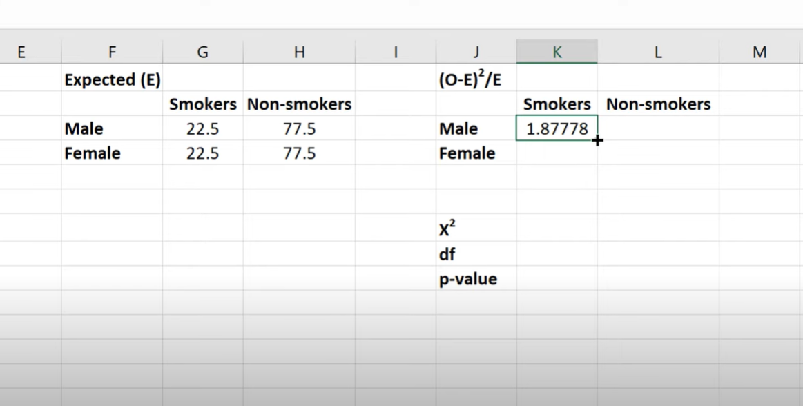
To calculate the chi-square test, you can use the following formula.
χ2 = Σ(Oi – Ei)2 / Ei
In this formula:
χ2 refers to the chi-square test statistic Oi stands for the observed frequency While Ei represents the expected frequency
how to do chi square in excel
The difference between the two is squared, summed and divided by the expected frequency. And by comparing the observed frequencies with the expected frequencies. The chi-square test statistic is then compared to a critical value to determine whether there’s a significant difference.
Performing the Chi-Square Test in Excel
To perform a chi-square test in Excel, you can take advantage of the built-in CHISQ.TEST function. Here is a guide on how to use it effectively.
First and foremost, you should enter your data into an Excel spreadsheet.
chi square analysis excel
Next, you will calculate the expected frequencies for each category. You can either do this manually. Or you can use utilize Excel’s CHISQ.INV.RT function to compute the expected frequencies automatically. After calculating the expected frequencies, you will use the CHISQ.TEST function to determine the chi-square test statistic.
The function takes two arguments. First is the range of cells containing the observed frequencies. And second one is the range of cells with expected frequencies. The result will be the chi-square test statistic.
how to do a chi square test in excel: What is chi square symbol
Now, you should compare the chi-square test statistic to the critical value. If the chi-square test statistic is greater than the critical value, then the difference between the expected and observed frequencies is significant.
Conclusion on formula for chi square test and how to compute chi square
In conclusion, a chi-square test is a easy functiın for analyzing categorical data.
Excel has CHISQ.TEST to perform the chi-square test quickly by yourself. If you well understand how the chi-square test works and how to perform it in Excel, you can analyze your data more effectively.
How to conduct a Chi-Square Test in Excel?
If you wish to make a Chi-Square Test in Excel, there are a few steps tough. First of all, it is essential to understand Chi-square test determines whether there is a significant difference between the expected and observed frequencies.
The p-value determines the probability of obtaining a test statistic as extreme as the one observed. This is assuming that the null hypothesis is true. The null hypothesis for the Chi-square test means there is no difference between the expected and observed frequencies. In contrast, the alternative hypothesis states there is a significant difference.
Alpha value and P-value
The likelihood of getting observed result in a set of data is represented by the p-value in a chi-square test. In a chi-square test, this value is usually compared to the alpha value. The likelihood you reject a null hypothesis when it is true is known as the alpha value. This indicates that obtaining a data set’s alpha value is less common than obtaining the p-value.
Chi-Square Test in Excel
Real-Life Example Of Chi-Square Test in Excel
First thing as an example, you gather sales data from the past six months and categorize it according to the product type. Such as Product A, B, or C and the geographic region where the sales are. Such as East, West or South. You will first fill this data into Excel and then, you can run the chi-square test.
The results show that there is a significant association between product type and geographic region (p < 0.05). Specifically, Product A is more popular in the East and West regions. While Product B is more popular in the South region. Product C tough shows no significant differences in popularity across regions.
how to do a chi square test in excel here
Accordingly, you can advise the client. And they can tailor their marketing strategies to each region accordingly. For instance, they should focus on promoting Product A in the East and West. While they should do the same for Product B in the South.
Additionally, you suggest they consider each region’s demographic characteristics when developing their marketing campaigns. Because the preferences of consumers in each region may vary.
chisq.test in excel
So when you got some points from your test, you provide the client with a summary of the chi-square results. After that, you can explain the implications for their business. You may say while there are clear regional differences in product popularity, they should also consider that some customers may purchase both Product A and B or neither of them.
Whether they choose to implement your suggestions is up to them tough. But with the data analysis you have, they have a solid foundation for making decisions.

A dedicated Career Coach, Agile Trainer and certified Senior Portfolio and Project Management Professional and writer holding a bachelor’s degree in Structural Engineering and over 20 years of professional experience in Professional Development / Career Coaching, Portfolio/Program/Project Management, Construction Management, and Business Development. She is the Content Manager of ProjectCubicle.